- Joined
- 9/22/20
- Messages
- 6
- Points
- 13
The price of a commodity can be described by the Schwartz mean reverting SDE
\[ dS = \alpha(\mu-\log S)Sdt + \sigma S dW \] where W is the standard Brownian motion and alpha is the strength of mean reversion.
From it is possible to derive the PDE for the price of the forward contract having the commodity as underlying asset
\[ (1) \qquad \frac{\partial F}{\partial t} + \alpha\Big(\mu-\frac{\mu-r}\alpha -\log S\Big)S\frac{\partial F}{\partial S}+\frac12\sigma^2S^2\frac{\partial^2F}{\partial S^2} = 0 \] whose analytical solution is \[ F(S,\tau)=\exp\bigg(e^{-\alpha\tau}\log S +\Big(\mu-\frac{\sigma^2}{2\alpha}-\frac{\mu-r}{\alpha}\Big)(1-e^{-\alpha\tau})+\frac{\sigma^2}{4\alpha}(1-e^{-2\alpha\tau})\bigg) \] where \(\tau=T-t\) is the time to expiry (\(T\) is the time of delivery/expiry).
Using Euler explicit method, i.e. forward difference on \(\dfrac{\partial F}{\partial t}\) and central difference on \(\dfrac{\partial F}{\partial S}\) and \(\dfrac{\partial^2F}{\partial S^2}\), we can discretize eq (1) as
\[ F^{n+1}_i = a F^n_{i-1} + b F^n_i + c F^n_{i+1} \] where \(a = \dfrac{S\Delta t}{2\Delta S}\bigg(\alpha\mu-(\mu-r)-\alpha\log(S)-\dfrac{\sigma^2S}{\Delta S}\bigg)\), \(b = \bigg(1-\sigma^2S^2\dfrac{\Delta t}{\Delta S^2}\bigg)\) and \(c = \dfrac{S\Delta t}{2\Delta S}\bigg(-\alpha\mu+(\mu-r)+\alpha\log(S)-\dfrac{\sigma^2S}{\Delta S}\bigg)\).
To run Explicit Euler we have then to choose the number \(N\) of time steps, which also set \(\Delta t\) since \(\Delta t = T/N\), and the size of \(\Delta S\). Since the finite difference scheme divides the cartesian plane (time is the X-axis, and spot price is the Y-axis) in a grid, if we take more time steps and/or smaller \(\Delta S\) the grid will be more dense and the accuracy of the approximation should increase (provided that \( 0<\frac{\Delta t}{(\Delta S)^2}<\frac12 \)).
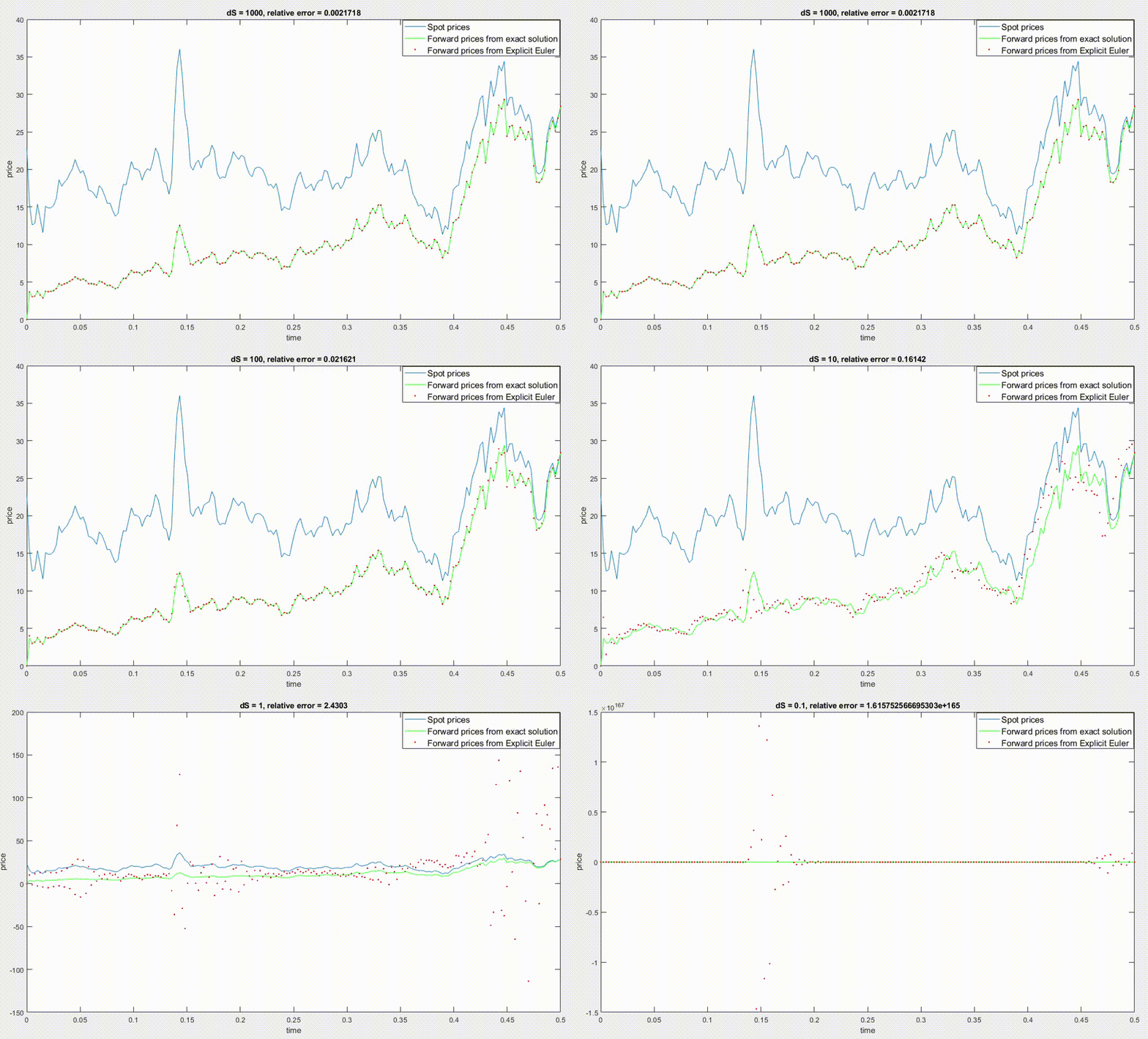
However, the code I wrote using the equations above doesn't work in this way, in particular to have big accuracy I have to use a large \(\Delta S\), and the accuracy decreses when using small values of \(\Delta S\) to point that by using \(\Delta S=0.1\) the relative error explodes to \(10^{165}\) as you can see in the image below (dS stands for \(\Delta S\)).
If you want you can inspect the matlab code (see attachment), I'm sure there is an error somewhere but cannot find it. I think one problem is the fact that I'm using real data (vector spot_prices in the code) and so I cannot discretize along the y-axis, right?
